Solve the infamous CGM98 problem using BayesCART

Tags: Bayesian CART, Tree models, MCMC

Categories: Blog, Coding, Tutorial

Bayesian CART with BayesCART: A Tutorial

Introduction

This tutorial introduces BayesCART, a Python package designed for Bayesian Classification and Regression Trees (CART) posterior sampling using advanced tempering methods. We demonstrate its functionality by solving the CGM98 example, originally introduced by Chipman et al. in 1998 [1]. This is a classical multimodal posterior sampling problem where standard MCMC methods struggle due to mode trapping.

Resources

• A theoretical treatment of Bayesian CART, and tempering algorithms
• The package documentation and official repo
• A discussion of the concept behind the creation of the package
• A notebook, with this code and somewhat fewer comments

Why Bayesian CART?

Classification and Regression Trees (CART) are powerful predictive models with intuitive interpretability. However, standard greedy algorithms often lead to suboptimal trees as they cannot recover from poor early splits. A Bayesian formulation introduces a prior over tree structures and leverages posterior inference to explore a more diverse set of trees while incorporating prior knowledge.

Bayesian CART faces a fundamental computational challenge: the posterior distribution over trees is highly multimodal, making Markov Chain Monte Carlo (MCMC) exploration inefficient. The BayesCART package addresses this by implementing customized tempering techniques to enhance sampling.

Installation

To install the package from source, run:

git clone https://github.com/guglielmogattiglio/bayescart.git
cd bayescart
pip install -e .

Imports

from joblib import Parallel, delayed
import numpy as np
from bayescart import BCARTClassic, NodeDataRegression, Tree, sim_cgm98
from bayescart import BCARTGeomLik, BCARTGeom, BCARTPseudoPrior
from bayescart.utils import plot_hists, plot_chain_comm, plot_swap_prob
from bayescart.eval import produce_tree_table
import pandas as pd
import matplotlib.pyplot as plt
from matplotlib.lines import Line2D

CGM98 Example

Theoretical Background

Consider the following setting, as in [1]:

\begin{equation} y = f(x_1, x_2) + 2\epsilon, \quad \epsilon \sim N(0,1) \end{equation}

with

\[f(x_1,x_2) = \begin{cases} 8.0 & \text{if } x_1 \leq 5.0 \text{ and } x_2 \in \{A,B\}\\ 2.0 & \text{if } x_1 > 5.0 \text{ and } x_2 \in \{A,B\}\\ 1.0 & \text{if } x_1 \leq 3.0 \text{ and } x_2 \in \{C,D\}\\ 5.0 & \text{if } 3.0< x_1 \leq 7.0 \text{ and } x_2 \in \{C,D\}\\ 8.0 & \text{if } x_1 > 7.0 \text{ and } x_2 \in \{C,D\} \end{cases}\]

The following Figure displays 800 iid observations drawn from this model.

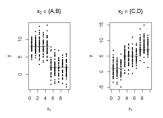
As the authors argue in their paper, this particular example tends to elude identification by greedy algorithms which minimize the residual sum of squares. The reason can be best seen below, where the response variable is plotted against the two predictors. The horizontal bars represent the mean response for the best split in $x_1$ plot, and mean levels for each value of $x_2$ in the other plot.

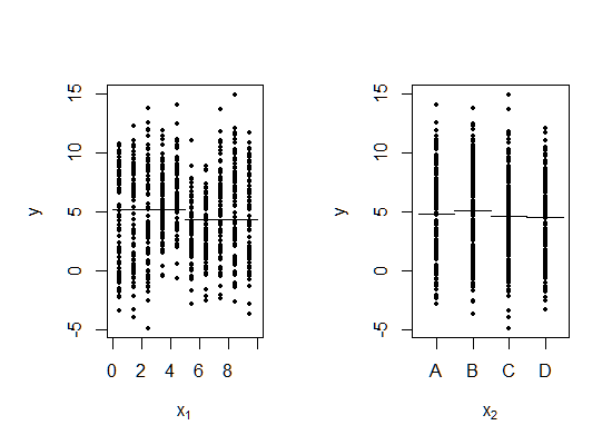
Note how a greedy procedure minimizing the RSS will prefer splitting on \(x_1\) at the root node, while the true tree splits along $x_2$ first.

Implementation

The CGM98 example is already implemented in the package. Let’s generate some data and construct the true tree using the package API. We’ll use the ground truth to compare its statistics, such as posterior probability and integrated likelihood values (based on the generated data), with the the MCMC sampler solution.

seed = 34647
rng = np.random.default_rng(seed)
X, y = sim_cgm98(800, rng)

Building the tree is simple and follows standard conventions. reset_split_info() is used to remove node parameters for leaf nodes, while update_subtree_data() partitions the dataset in root to each of the leaf nodes, based on the split structure that we have defined.

root_node_data = NodeDataRegression(np.nan, np.nan, X, y, rng=rng, debug=True, node_min_size=1)

true_tree = Tree(root_node_data=root_node_data, rng=rng, debug=True, node_min_size=1)
root = true_tree.get_root()
root.update_split_info('v2', ['a','b'])
root.update_node_params((np.nan, np.nan))
node2 = true_tree.add_node(root_node_data.copy(), is_l=True, parent=root)
node2.update_split_info('v1', 5)
node2.update_node_params((np.nan, np.nan))
node3 = true_tree.add_node(root_node_data.copy(), is_l=False, parent=root)
node3.update_split_info('v1', 3)
node3.update_node_params((np.nan, np.nan))
node4 = true_tree.add_node(root_node_data.copy(), is_l=True, parent=node2)
node4.update_node_params((8, 2))
node4.reset_split_info()
node5 = true_tree.add_node(root_node_data.copy(), is_l=False, parent=node2)
node5.update_node_params((2, 2))
node5.reset_split_info()
node6 = true_tree.add_node(root_node_data.copy(), is_l=True, parent=node3)
node6.update_node_params((1, 2))
node6.reset_split_info()
node7 = true_tree.add_node(root_node_data.copy(), is_l=False, parent=node3)
node7.update_split_info('v1', 7)
node7.update_node_params((np.nan, np.nan))
node8 = true_tree.add_node(root_node_data.copy(), is_l=True, parent=node7)
node8.update_node_params((5, 2))
node8.reset_split_info()
node9 = true_tree.add_node(root_node_data.copy(), is_l=False, parent=node7)
node9.update_node_params((8, 2))
node9.reset_split_info()

true_tree.update_subtree_data(root)

To check correctness, we can use the is_valid() function, which verifies all the logical components of the trees are consistent with one another.

true_tree.is_valid()

Finally, let’s run the sampler. The BCARTClassic class implements the original CGM98 posterior exploration algorithm, which runs multiple short chains that quickly converge on a mode and often get stuck. Once this happens, the sampler restarts from another random part of the space. Repeating this process aims to cover all the modes and, by chance, find the tree(s) with the highest posterior probability.

Limitations of the CGM98 Approach

• Lack of Posterior Sampling: This method does not provide a posterior sample, meaning we do not get a full collection of trees sampled from the posterior distribution.
• Difficulty in Identifying the Best Tree: The most frequently encountered tree does not inherently hold more significance. Instead, trees are compared using the integrated likelihood. Using posterior tree probabilities is discouraged (see the original paper for details).

While using the integrated log-likelihood is a reasonable approach, it falls short of a full Bayesian methodology. Essentially, this approach can be interpreted as a Bayesian-driven tree search, but tree evaluation still relies on classical statistics (e.g., the likelihood).

Note that, in theory, running the MCMC for longer and applying sufficient thinning will eventually yield a valid posterior sample. However, in practice, the algorithm struggles to escape locally optimal trees efficiently. This motivates the need for more sophisticated techniques, such as parallel tempering, to enhance posterior exploration.

def run_classic_MCMC(X, y, seed):
    bcart = BCARTClassic(X, y, alpha=0.95, beta=1, a=1/3, mu_bar=4.85, 
                         nu=10, lambd=4, iters=1010, burnin=10, thinning=4, 
                         move_prob=[1,1,1,1], light=False, seed=seed, verbose='')
    res = bcart.run()
    return res['posterior_store'], res['integr_llik_store'], res['tree_term_reg']

res = Parallel(-1)(delayed(lambda i: run_classic_MCMC(X, y, i))(seed+i) for i in range(10))
post, llik, term_reg = zip(*res)

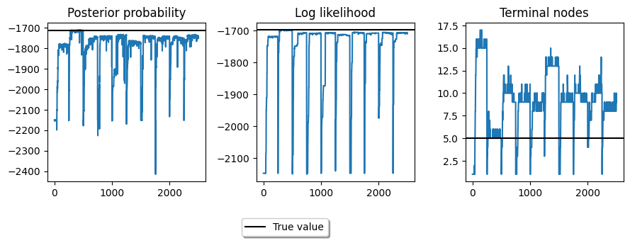
Let’s visualize the outcome. Below we aggregate each of the 10 independent runs in a single plot. The beginning of each run is clearly visible as when it resets, starting from a stump means that the metrics we use are usually pretty poor, until better trees are found by the sampler.

def unravel(l):
    out = []
    [out.extend(x) for x in l]
    return out

fig,ax = plt.subplots(1,3, figsize=(9,3)) 
ax[0].plot(unravel(post))
ax[0].axhline(true_post, color='black')
ax[0].set_title('Posterior probability')
ax[1].plot(unravel(llik))
ax[1].axhline(true_llik, color='black')
ax[1].set_title('Log likelihood')
ax[2].plot(unravel(term_reg))
ax[2].axhline(5, color='black')
fig.tight_layout()
ax[2].set_title('Terminal nodes')
ax[0].legend([Line2D([0],[0],c='black')], ['True value'], 
             loc='upper center', bbox_to_anchor=(1.5, -0.2), 
             ncol=1, fancybox=True, shadow=True)

Parallel Tempering

Parallel tempering enhances posterior exploration in Bayesian models with multimodal distributions. It runs multiple MCMC chains in parallel, each targeting a flattened version of the posterior. These chains probabilistically exchange states, helping the primary chain escape local modes and explore more effectively.

Flatter distributions allow freer movement across modes but reduce the ability to distinguish high- from low-probability regions. However, swapping with chains closer to the original posterior helps retain accuracy while improving traversal.

Types of Parallel Tempering

BayesCART implements three tempering strategies:

• Geometric Tempering: Flattens the posterior using a temperature schedule, similar to simulated annealing.
• Geometric-Likelihood Tempering: Applies temperature scaling only to the likelihood, letting the prior retain its influence, which biases exploration toward smaller trees.
• Pseudo-Prior Tempering: Uses an auxiliary pseudo-prior to guide exploration toward certain tree sizes while preserving the original prior.

For a theoretical treatment of each of these tempering types, refer to this in-depth series.

Simulation Setup

We run eight independent simulations per method, each with a different random initialization. If all chains behave similarly, they are likely covering the posterior well; if they sample vastly different trees, it signals poor mixing.

Each method runs an equivalent number of total MCMC steps, but parallel tempering distributes these across chains, reducing direct updates per chain while improving overall exploration.

For this study:

• Geometric tempering uses 8 chains.
• Geometric-likelihood and pseudo-prior tempering use 4 chains each.
• Temperatures are tuned for optimal swap acceptance rates to ensure overlap.

While maintaining multiple chains increases computational cost, the improved posterior coverage and mode traversal justify the trade-off, particularly for Bayesian CART models where standard MCMC struggles with multimodal distributions.

Note: Simulation runtimes vary based on hardware, typically ranging from 20 minutes to several hours per experiment.

base_iter = 50000
base_burnin = 1000
thinning_base = 20
tree_spacing_base = 20

def run_classic_MCMC(X, y, seed):
    mult = 8
    bcart = BCARTClassic(X, y, alpha=0.95, beta=1, a=1/3, 
                         mu_bar=4.85, nu=10, lambd=4, 
                         iters=mult*base_iter, burnin=mult*base_burnin, 
                         thinning=mult*thinning_base, move_prob=[1,1,1,1], 
                         light=False, seed=seed, verbose='', 
                         store_tree_spacing=mult*tree_spacing_base)
    return bcart.run()

def run_geom_tempering(X, y, seed):
    mult = 1
    bcart = BCARTGeom(X, y, alpha=0.95, beta=1, a=1/3, mu_bar=4.85, 
                      nu=10, lambd=4, iters=mult*base_iter, 
                      burnin=mult*base_burnin, thinning=mult*thinning_base, 
                      move_prob=[1,1,1,1], light=False, seed=seed, 
                      temps = (1,0.85, 0.7,0.48,0.31,0.2,0.08,1e-7), verbose='', 
                      store_tree_spacing=mult*tree_spacing_base)
    return bcart.run()

def run_geom_lik_tempering(X, y, seed):
    mult =  2
    bcart = BCARTGeomLik(X, y, alpha=0.95, beta=1, a=1/3, mu_bar=4.85, nu=10, 
                         lambd=4, iters=mult*base_iter, burnin=mult*base_burnin, 
                         thinning=mult*thinning_base, move_prob=[1,1,1,1], 
                         light=False, seed=seed, temps = (1, 0.04, 0.011, 0.005), 
                         verbose='', store_tree_spacing=mult*tree_spacing_base)
    return bcart.run()

def run_pseudo_prior_tempering(X, y, seed):
    mult= 2 
    bcart = BCARTPseudoPrior(X, y, alpha=0.95, beta=1, a=1/3, mu_bar=4.85, nu=10, 
                             lambd=4, iters=mult*base_iter, burnin=mult*base_burnin, 
                             thinning=mult*thinning_base, move_prob=[1,1,1,1], 
                             light=False, seed=seed, temps = (1, 0.065, 0.028, 0.015), 
                             verbose='', store_tree_spacing=mult*tree_spacing_base, 
                             pprior_alpha=0.95, pprior_beta=1.6)
    return bcart.run()

seed = 34647
rng = np.random.default_rng(seed)
X, y = sim_cgm98(800, rng)

res_classic = list(Parallel(-1)(delayed(lambda i: run_classic_MCMC(X, y, i))(seed+i) for i in range(8)))
res_geom = list(Parallel(-1)(delayed(lambda i: run_geom_tempering(X, y, i))(seed+i) for i in range(8)))
res_geom_lik = list(Parallel(-1)(delayed(lambda i: run_geom_lik_tempering(X, y, i))(seed+i) for i in range(8)))
res_pp = list(Parallel(-1)(delayed(lambda i: run_pseudo_prior_tempering(X, y, i))(seed+i) for i in range(8)))

mdls = [res_classic, res_geom, res_geom_lik, res_pp]

# relatively expensive to run, the implementation is not parallelized
summary_tbls = [produce_tree_table(res) for res in mdls]

Notice the sensible gains in runtime for geometric-likelihood and pseudo-prior approaches. That is due to the exploration of smaller trees, that are computationally cheaper. This is more pronounced the bigger the dataset.

names = ['Classic MCMC', 'Geometric Tempering', 'Geometric Likelihood Tempering', 'Pseudo Prior Tempering']
for res, name in zip(mdls, names):
    timings = res[0]['timings']
    print(f'{name}. \nElapsed time: {timings["elap_time_human"]}, Tot iters: {timings["tot_mh_steps"]}, Iters/min: {timings["iters/min"]}/min')

Classic MCMC. 
Elapsed time: 6 minutes and 49 seconds, Tot iters: 400000, Iters/min: 58613/min
Geometric Tempering. 
Elapsed time: 8 minutes and 21 seconds, Tot iters: 50000, Iters/min: 5984/min
Geometric Likelihood Tempering. 
Elapsed time: 5 minutes and 16 seconds, Tot iters: 100000, Iters/min: 18972/min
Pseudo Prior Tempering. 
Elapsed time: 5 minutes and 32 seconds, Tot iters: 100000, Iters/min: 18041/min

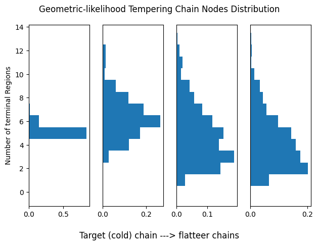
Checking chain alignment

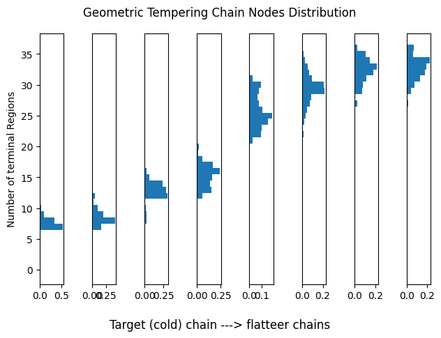
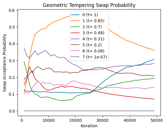
Let us assess the current temperature setup for tempering. Each histogram represents the distribution of terminal regions for a given chain. As remarked, we want chains to partially overlap to encourage more frequent swaps. For this analysis we will consider only one run of each algorithm.

Geometric Tempering

plot_chain_comm(res_geom[0], title='Geometric Tempering Chain Nodes Distribution') 
plot_swap_prob(res_geom[0], title='Geometric Tempering Swap Probability')

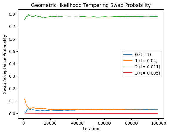
Geometric-Likelihood Tempering

plot_chain_comm(res_geom_lik[0], title='Geometric-likelihood Tempering Chain Nodes Distribution') 
plot_swap_prob(res_geom_lik[0], title='Geometric-likelihood Tempering Swap Probability')

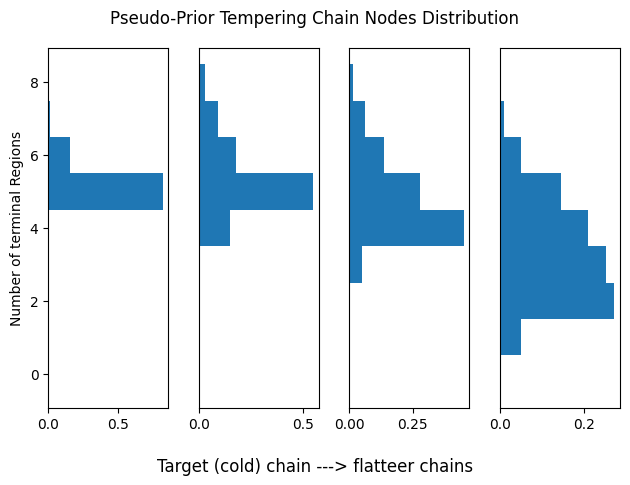
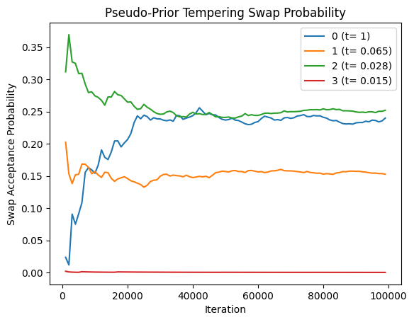
Pseudo-Prior Tempering

plot_chain_comm(res_pp[0], title='Pseudo-Prior Tempering Chain Nodes Distribution') 
plot_swap_prob(res_pp[0], title='Pseudo-Prior Tempering Swap Probability')

Assessing tempering performance

We use two indicators of performance. First, we would want the marginal distribution of features of interest to be consistent across runs. For this, we consider the number of terminal regions. While this does not guarantee convergence, terminal regions are usually a good proxy of at least identifying good trees.

The rigorous (and far stricter) test is to compare the posterior probability of the same tree across runs. A sampler that mixes well will be able to identify the same high posterior trees in all runs. This is represented in the table. Note that a value of zero means the given tree was sampled $< 1\%$.

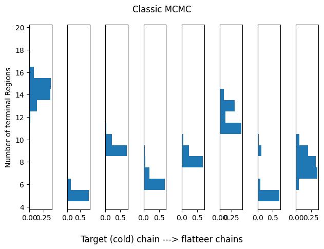
Classic CGM98 MCMC Sampler

We use this as a baseline for tempering, even though we know it will struggle.

idx_range = (0,1)
plot_hists(res_classic, idx_range=idx_range, title='Classic MCMC')
print(summary_tbls[0][:5])

	C0	C1	C2	C3	C4	C5	C6	C7	Mn	Std	b
0	0.0	0.85	0.0	0.0	0.00	0.0	0.87	0.00	0.22	0.37	5.0
1	0.0	0.00	0.0	0.8	0.00	0.0	0.00	0.06	0.11	0.26	6.0
2	0.0	0.00	0.0	0.0	0.00	0.0	0.00	0.42	0.05	0.14	7.0
3	0.0	0.00	0.0	0.0	0.39	0.0	0.00	0.00	0.05	0.13	8.0
4	0.0	0.00	0.0	0.0	0.34	0.0	0.00	0.00	0.04	0.11	8.0

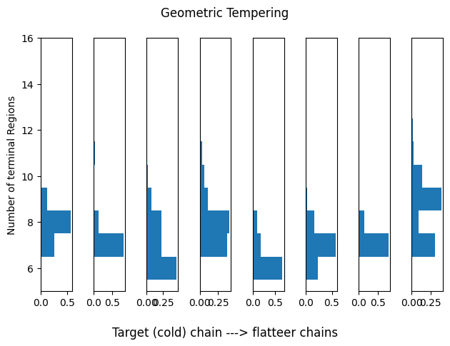
Geometric Tempering

Our off-the-shelf tempering-based sampler. Notice how this tends to focus on extremely large trees on flatter landscapes (warmer chains).

idx_range = (0,1)
plot_hists(res_geom, idx_range=idx_range, title='Geometric Tempering')
print(summary_tbls[1][:5])

	C0	C1	C2	C3	C4	C5	C6	C7	Mn	Std	b
0	0.00	0.0	0.55	0.00	0.7	0.28	0.00	0.00	0.19	0.27	6.0
1	0.32	0.0	0.00	0.00	0.0	0.00	0.00	0.38	0.09	0.15	7.0
2	0.00	0.0	0.00	0.00	0.0	0.00	0.00	0.36	0.04	0.12	9.0
3	0.00	0.0	0.00	0.26	0.0	0.00	0.00	0.00	0.03	0.09	7.0
4	0.00	0.0	0.00	0.00	0.0	0.00	0.22	0.00	0.03	0.07	7.0

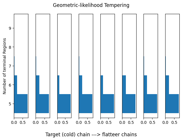
Geometric-likelihood Tempering

This works much better! However, we can get better results by disentangling the prior distribution and flattening the full posterior instead of only the likelihood.

idx_range = (0,1)
plot_hists(res_geom_lik, idx_range=idx_range, title='Geometric-likelihood Tempering')
print(summary_tbls[2][:5])

	C0	C1	C2	C3	C4	C5	C6	C7	Mn	Std	b
0	0.77	0.72	0.85	0.78	0.81	0.81	0.76	0.74	0.78	0.04	5.0
1	0.02	0.02	0.02	0.01	0.02	0.02	0.02	0.02	0.02	0.00	6.0
2	0.00	0.07	0.00	0.03	0.00	0.00	0.00	0.03	0.02	0.02	6.0
3	0.01	0.01	0.02	0.02	0.01	0.02	0.01	0.02	0.02	0.00	6.0
4	0.03	0.00	0.00	0.00	0.02	0.01	0.02	0.03	0.01	0.01	6.0

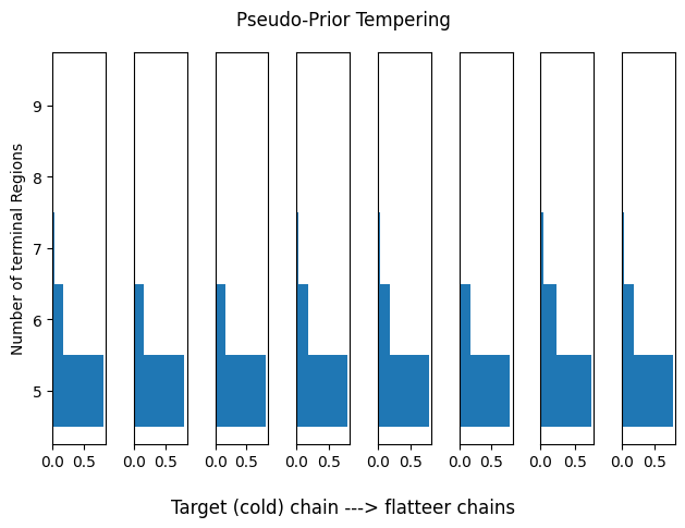
Pseudo-Prior Tempering

We observe clear converge, both in terms of the marginal over the terminal regions, and through the estimated posterior probabilities.

idx_range = (0,1)
plot_hists(res_pp, idx_range=idx_range, title='Pseudo-Prior Tempering')
print(summary_tbls[3][:5])

	C0	C1	C2	C3	C4	C5	C6	C7	Mn	Std	b
0	0.80	0.81	0.80	0.83	0.80	0.79	0.72	0.78	0.79	0.03	5.0
1	0.01	0.01	0.02	0.01	0.02	0.02	0.02	0.02	0.02	0.00	6.0
2	0.02	0.02	0.02	0.01	0.02	0.01	0.01	0.01	0.02	0.00	6.0
3	0.01	0.01	0.01	0.01	0.02	0.01	0.01	0.01	0.01	0.00	6.0
4	0.01	0.01	0.01	0.01	0.01	0.01	0.02	0.01	0.01	0.00	6.0

References

[1] Chipman, H. A., George, E. I., & McCulloch, R. E. (1998). Bayesian CART model search. Journal of the American Statistical Association, 93(443), 935–948.